


Programming Projects:
Local Spin-Density Approximations in KS-DFT
contributed by Sina Mostafanejad
Local Spin-Density Approximations in KS-DFT
contributed by Sina Mostafanejad
Overview
The Kohn-Sham density functional theory (KS-DFT) relies on the approximate forms of the exchange-correlation (XC) energy density functionals to predict the electronic structure of various many-body systems. Therefore, gaining a minimum-level background and basic knowledge about the underlying theories and details of about their implementation is important. This tutorial is focused on one of the simplest class of approximations in KS-DFT: the local spin-density approximation (LSDA). In case one deals with a restricted closed-shell system, LSDA is called LDA. The LDA (LSDA) functionals solely depend on the local value of the density ρ(r) (or spin-densities ρα and ρβ) at each point r in space.
This tutorial assumes that you are familiar with the SCF procedure in general and have completed the previous restricted Hartree-Fock (RHF) tutorial that employed the JK object. Since we develop the LSDA plugin based on the unrestricted Kohn-Sham (UKS) DFT tutorial, you should also make yourself familiar with it before you get started.
The C++ and Python code for this LDA plugin can be found here.
The Exchange-Correlation Functional
Note: we use atomic units throughout this tutorial.
In KSDFT, the electronic energy is a universal functional of the one-electron density. There does also exist a fictitious noninteracting system of electrons that has the same density as the true set of electrons. The states of the fictitious system are determined in a manner that is similar to Hartree-Fock theory; the Kohn-Sham wave function is a single antisymmetrized product of Kohn-Sham orbitals, and these orbitals are determined as the eigenvectors of an effective one-electron operator that accounts for true many-body effects. The UKS energy is

where Exc represents the XC energy functional, and ρα and ρβ represent the α and β spin densities, respectively. These spin densities are the real-space representation of the densities, defined as
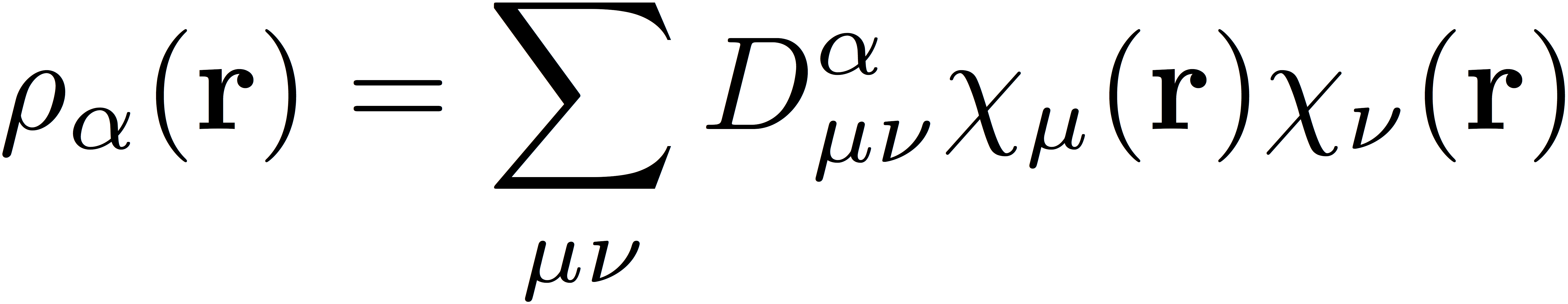
and

As briefly mentioned in the introduction, the simplest class of functionals are the LSDA XC functionals. One of the most popular XC functionals in the literature is the combination of Slater (S) or Slater-Dirac exchange and Vosko-Wilk-Nusair expression III (VWN3) correlation functional, which is called SVWN3. In this tutorial, we focus on building the exchange part of this functional. The interested reader may find the implementation of the VWN3 correlation functional in the provided plugin folder.
The Slater exchange functional ESx[ρσ(r)] is defined as sum of the individual exchange contribution from each spin-density ρσ where σ can represent α or β spin
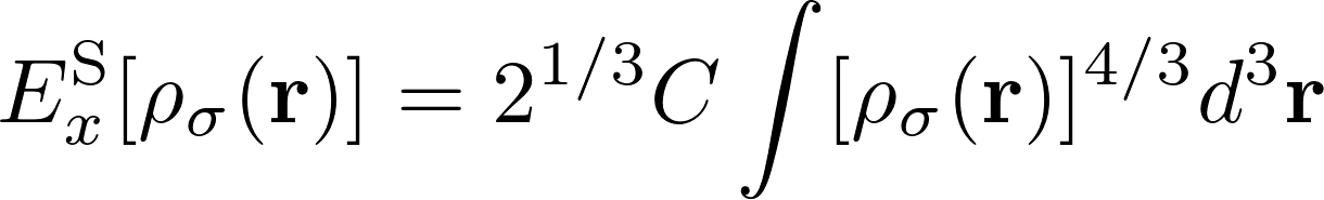
where the coefficient C is defined as
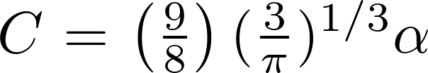
in which, α is equal to (2/3). Therefore, the Slater exchange functional ESx[ρα(r),ρβ(r)] can be expressed as

Calculating the Integrals: Quadrature Methods
In order to calculate the value of the integrals numerically, there are various techniques that one can use. Numerical quadrature methods are one of the most popular methods for approximating the integrals with low dimension(s). For higher dimensions, one usually resorts to other numerical techniques such as Monte Carlo.
Back to our integral expression in the definition of the Slater exchange functional, one can adopt the quadrature approach to come up with an approximation to recast the integral expression into
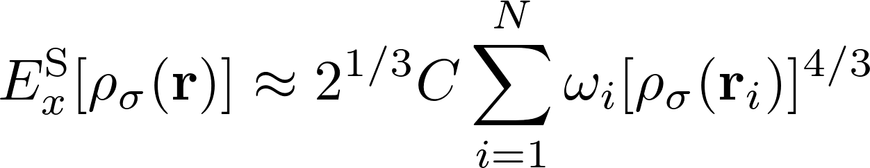
where, ωi is the weight factor at each point ri. In simple terms, we have broken the integral into a sum of N instances of the function, calculated at each of the N points, ri weighted by ωi. For this reason, this technique is often called an N-point quadrature.
One usually seeks to find optimal points to maximize the efficiency of the numerical estimatation of the integral. Fortunately, we do not have to worry about the technicalities of the fundamental theorem of Gaussian quadrature to find the optimal points or look them up in tables to calculate the quadrature summation. Psi4 provides us with the standard Lebedev-Laikov spherical quadratures which is an extremely efficient method and is based on the conventional atomic partitioning schemes. The resolution of this spherical grid can be controlled via DFT_SPHERICAL_POINTS option in the input file. For further details on possible values of this option see here.
Implementation of the DFT Grids
Working with grids and DFT quadrature starts by including the pertinent header files in your plugin code. The header files give you access to the functions you need to build the quadrature.
    // for DFT grids
    #include "psi4/libfock/points.h"
    #include "psi4/libfock/cubature.h"
In order to initialize the grids, one way is to read the information from the reference KS-DFT wave function.
    // read in a reference wave function from a previous dft job
    scf::HF* scfwfn = (scf::HF*)reference_wavefunction_.get();
    std::shared_ptr functional = scfwfn->functional();
    std::shared_ptr potential = scfwfn->V_potential();
The next step is to compute the grid points ri and calculate the values of the orbitals on each of these points, φ(ri), on the mesh. Note that Psi4 stores the mesh of grid points in a block strucure. Thus, to determine the number of blocks (nblocks), the number of grid points in each block (npoints), and the total number of grid points (phi_points_), we proceed as shown below
    // since grid is stored in blocks, we need to build a full phi matrix
    // from the individual blocks:
    std::shared_ptr points_func = potential->properties()[0];
    points_func->set_pointers(Da_,Db_);

    // determine number of grid points
    int nblocks = potential->nblocks();
    phi_points_       = 0;
    int max_functions = 0;
    int max_points    = 0;
    for (int myblock = 0; myblock < nblocks; myblock++) {
        std::shared_ptr block = potential->get_block(myblock);
        points_func->compute_points(block);
        int npoints = block->npoints();
	phi_points_ += npoints;

        // phi matrix (real-space <- AO basis mapping)
        const std::vector& function_map = block->functions_local_to_global();
        int nlocal = function_map.size();
        if ( nlocal > max_functions ) max_functions = nlocal;
        if ( npoints > max_points )   max_points    = npoints;
    }
We now need to implement a function, say, BuildPhiMatrix(), that builds the super-phi matrix, Φpxn, which includes the values of n orbitals φ(ri) calculated on a mesh of p grid points. The details of the BuildPhiMatrix() can be coded in three steps as follows
    void DFTSolver::BuildPhiMatrix(std::shared_ptr potential,
                                   std::shared_ptr points_func,
                                   std::string phi_type, std::shared_ptr myphi) {

    // STEP I: Count the number of grid points and blocks
    int nblocks = potential->nblocks();

    phi_points_ = 0;
    for (int myblock = 0; myblock < nblocks; myblock++) {
        std::shared_ptr block = potential->get_block(myblock);
        points_func->compute_points(block);
        int npoints = block->npoints();
        const std::vector& function_map = block->functions_local_to_global();
        int nlocal = function_map.size();


	/*   STEP II: Define and store the weight factors and the coordinates
	 *   of the grid points in vectors grid_w_, grid_x_ etc. and the
         */  values of the basis functions phi(r) at each point in a matrix

        double ** phi = points_func->basis_value(phi_type)->pointer();

        double * x = block->x();
        double * y = block->y();
        double * z = block->z();
        double * w = block->w();

        for (int p = 0; p < npoints; p++) {

            grid_x_->pointer()[phi_points_ + p] = x[p];
            grid_y_->pointer()[phi_points_ + p] = y[p];
            grid_z_->pointer()[phi_points_ + p] = z[p];
            grid_w_->pointer()[phi_points_ + p] = w[p];

            for (int nu = 0; nu < nlocal; nu++) {
                int nug = function_map[nu];
                myphi->pointer()[phi_points_ + p][nug] = phi[p][nu];
            }
        }
        phi_points_ += npoints;
    }

    // STEP III: Transformation of the orbitals from AO to SO basis

    // grab AO->SO transformation matrix
    std::shared_ptr ao2so = reference_wavefunction_->aotoso();

    // transform one index of super phi matrix (AO->SO)
    std::shared_ptr temp (new Matrix(myphi));

    for (int p = 0; p < phi_points_; p++) {
        for (int sigma = 0; sigma < nso_; sigma++) {
            double dum = 0.0;
            for (int nu = 0; nu < nso_; nu++) {
                dum += myphi->pointer()[p][nu] * ao2so->pointer()[nu][sigma];
            }
            temp->pointer()[p][sigma] = dum;
        }
    }
We can now declare our cooridante vectors and basis matrices in the main code (here, as class variables) and call our BuildPhiMatrix() function to store all the ingredients into their corresponding memory addresses.
    // declaring our class variables for storing the weights and coordinates
    // of our grid points into their corresponding vectors and matrix containers

    super_phi_   = std::shared_ptr(new Matrix("SUPER PHI",phi_points_,nso_));

    grid_x_      = std::shared_ptr(new Vector("GRID X",phi_points_));
    grid_y_      = std::shared_ptr(new Vector("GRID Y",phi_points_));
    grid_z_      = std::shared_ptr(new Vector("GRID Z",phi_points_));
    grid_w_      = std::shared_ptr(new Vector("GRID W",phi_points_));

    // build the super_phi matrix
    BuildPhiMatrix(potential, points_func, "PHI",  super_phi_);
Spin-Density Functions
The next step is to use the aforementioned expressions for building the spin-density functions from reduced-density matrices (Da and Db) . Similar to the BuildPhiMatrix() function , we can define BuildRho() as
    void DFTSolver::BuildRho(std::shared_ptr Da, std::shared_ptr Db) {

        rho_a_   = (std::shared_ptr)(new Vector(phi_points_));
        rho_b_   = (std::shared_ptr)(new Vector(phi_points_));

        rho_   = (std::shared_ptr)(new Vector(phi_points_));

        double ** phi   = super_phi_->pointer();
        double ** Dap = Da->pointer();
        double ** Dbp = Db->pointer();

        double * rho_ap = rho_a_->pointer();
        double * rho_bp = rho_b_->pointer();

        double * rho_p = rho_->pointer();

        for (int p = 0; p < phi_points_; p++) {
            double duma   = 0.0;
            double dumb   = 0.0;
            for (int sigma = 0; sigma < nso_; sigma++) {
                for (int nu = 0; nu < nso_; nu++) {
                    duma += phi[p][sigma] * phi[p][nu] * Dap[sigma][nu];
                    dumb += phi[p][sigma] * phi[p][nu] * Dbp[sigma][nu];
                }
            }
            rho_ap[p] = duma;
            rho_bp[p] = dumb;

            rho_p[p] = rho_ap[p] + rho_bp[p];
        }
    }
Since the orbitals are built on the mesh of p grid points, one obtains p instances of the function ρσ(ri) calculated on the grid points ri. The calculated values of the density function can be stored in the corresponding vectors (which again, can be declared as class variables) rho_a_ and rho_b_.
Implementation of the Exchange Functional
Armed with all the ingredients we need to approximate the integrals in the Slater exchange functional ESx[ρσ(r)] expression, we can start implementing our functional as
    double DFTSolver::EX_LSDA_I(std::shared_ptr rho_a, std::shared_ptr rho_b){

        const double alpha = (2.0/3.0);      // Slater value
        const double Cx = (9.0/8.0) * alpha * pow(3.0/M_PI,1.0/3.0);

        double * rho_ap = rho_a->pointer();
        double * rho_bp = rho_b->pointer();

        double exc = 0.0;
        for (int p = 0; p < phi_points_; p++) {

            double exa = pow(2.0,1.0/3.0) * Cx * pow( rho_ap[p], 4.0/3.0) ;
            double exb = pow(2.0,1.0/3.0) * Cx * pow( rho_bp[p], 4.0/3.0) ;
            double ex_LSDA = exa + exb;
            exc += - ex_LSDA * grid_w_->pointer()[p];
        }
        return exc;
The total KS energy is the sum of the non-interacting kinetic energy , nuclear-attraction and classical Coulomb energy as well as the exchange and correlation energy contributions. The details for obtaining the first three terms is shown in the UKS tutorial. Here, we show how to implement and call the Slater exchange energy function EX_LSDA_I()
        e_current  = enuc_;
        e_current += one_electron_energy;
        e_current += two_electron_energy;

        // calculating the LDA energy w/ our LDA exchange functional
        // E = H + J + E_X
        e_lda = e_current;
        e_lda += EX_LSDA_I(rho_a_,rho_b_);

        /* NOTE: we have to add the whole EXC first since in the new libxc
           we apparently do not have the Slater-Dirac's Ex function separately.
           Therefore, we have to call the whole XC energy and then subtract EC
           that we have written manually from it.
        */

        // calculating the LDA energy using Psi4's built-in functional
        // E = H + J + E_XC - EC
        e_current += exchange_correlation_energy;
        e_current -= EC_VWN3_RPA_III(rho_a_,rho_b_);
Which yields the following output for the ground-state of the water molecule within the STO-3G basis
    ==>  Begin SCF Iterations <==

     Iter               energy                   dE          RMS |[F,P]|
        0     -72.217789121887      46.090441606660       0.160193268072
        1     -73.451287273904      -1.233498152018       0.127193144590
        2     -73.691444981154      -0.240157707250       0.096756216936
        3     -73.828025256035      -0.136580274881       0.082325141465
        4     -74.032633899725      -0.204608643689       0.004615876139
        5     -74.032705396426      -0.000071496702       0.000896622578
        6     -74.032594885610       0.000110510816       0.000014180596
        7     -74.032592609581       0.000002276029       0.000000868197
        8     -74.032592742227      -0.000000132646       0.000000001744
        9     -74.032592741964       0.000000000262       0.000000003456
       10     -74.032592741970      -0.000000000006       0.000000003419
       11     -74.032592742491      -0.000000000521       0.000000000002
       12     -74.032592742491       0.000000000000       0.000000000000

    SCF iterations converged!

    * SCF total energy:     -74.032592742491
    * LDA total energy:     -74.032592742491
In the present tutorial, We did not talk about the details of the implementation of the correlation functional EC_VWN3_RPA_III(). Therefore, the next challenge would be to refer to the literature and try to understand the fundamentals and the details of the implementation of the VWN3 correlation functional included in the plugin's code.