


Programming Projects: Unrestricted Kohn-Sham DFT
Overview
In this project, you will develop an unrestricted Kohn-Sham (UKS) DFT code as a plugin to the Psi4 electronic structure package. We will first develop an unrestricted Hartree-Fock (UHF) algorithm using the JK object in Psi4, which is capable of building coulomb-like (J) and exchange-like (K) matrices for arbitrary densities. Then, we will use Psi4's DFT functional and potential objects to turn the UHF code into a UKS DFT code. This tutorial assumes that you are familiar with the SCF procedure in general and have completed the previous restricted Hartree-Fock (RHF) tutorial that employed the JK object.
The C++ and Python code for this UKS plugin can be found here.
Unrestricted Hartree Fock
Note: we use atomic units throughout this tutorial.
The previous Hartree-Fock tutorials introduced the idea of restricted Hartree-Fock theory, where it is assumed that the α- and β-spin orbitals (and density matrices, Fock matrices, etc.) are the same. These assumptions simplify the self-consistent field (SCF) procedure. Here, we lift that assumption and employ unrestricted Hartree-Fock theory, where α- and β-spin orbitals can be different. At the UHF level of theory, the total electronic energy is given by
where h represents the core Hamiltonian matrix, Dα and Dβ represent the density matrices for α- and β-spin electrons, respectively, and Fα and Fβ represent the Fock matrices for α- and β-spin electrons, respectively. Here, the indices μ and ν represent atomic orbital (AO) basis functions. As in the previous tutorials, the core Hamiltonian matrix is comprised of integrals that represent both the electron kinetic energy and the electron-nuclear potential energy, and the atomic orbital basis functions are not orthogonal.
The α- and β-spin Fock matrices are defined as
and
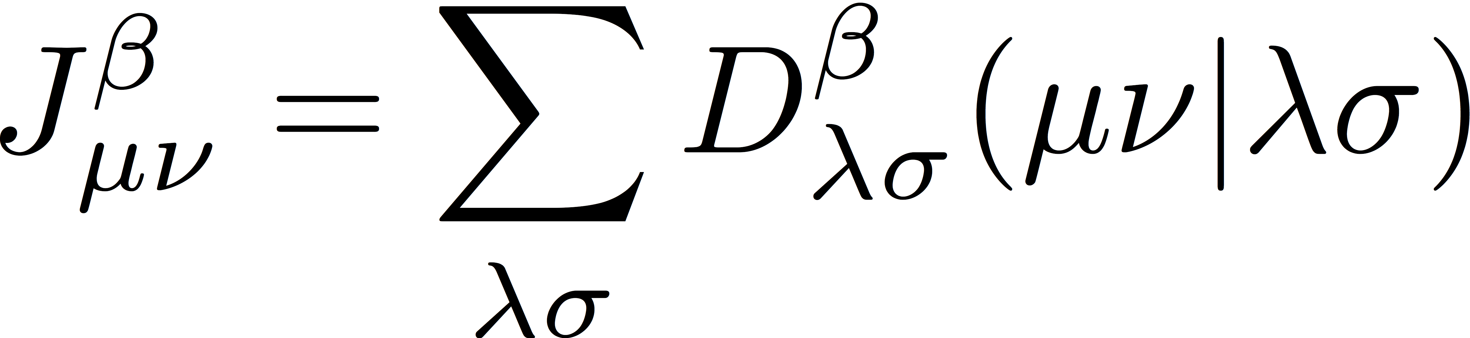
where Jα and Jβ are Coulomb matrices for α- and β-spin electrons, respectively, defined as
and
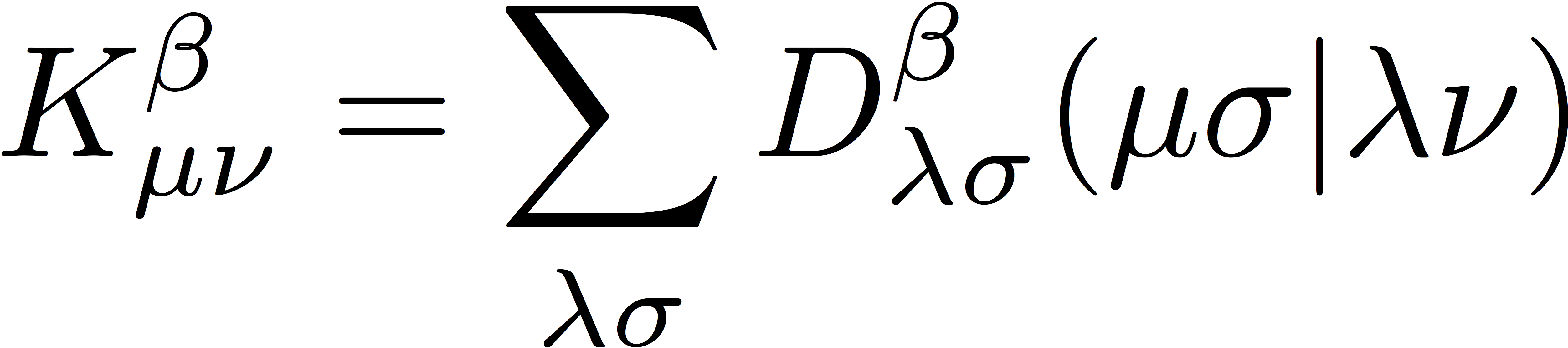
Similarly, we define exchange matrices for α- and β-spin electrons as
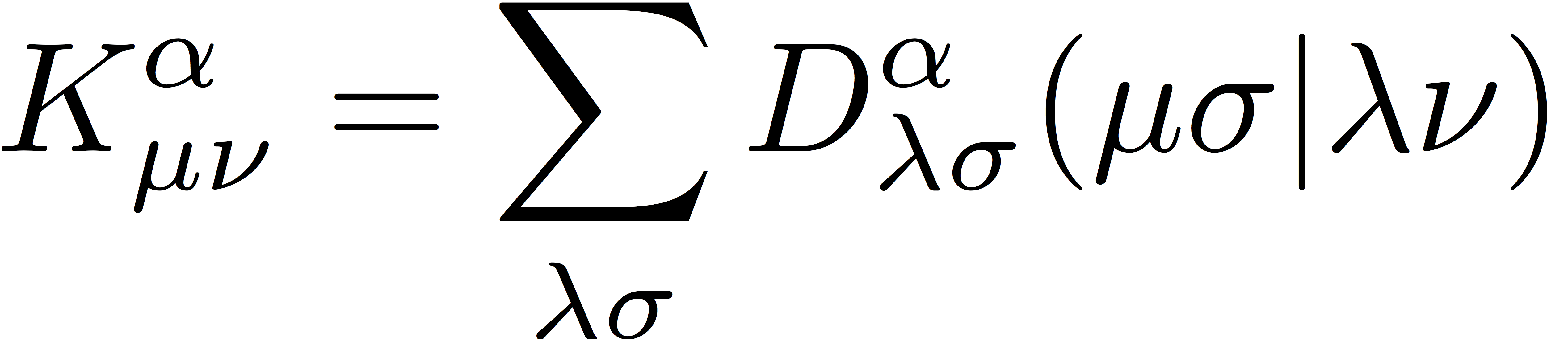
and
As in RHF, the UHF wave function is an antisymmetrized product of N molecular orbitals (MOs), and the energy is minimized with respect to variations in the shape of these MOs. We separately expand the α- and β-spin orbitals as linear combinations of atomic orbitals as
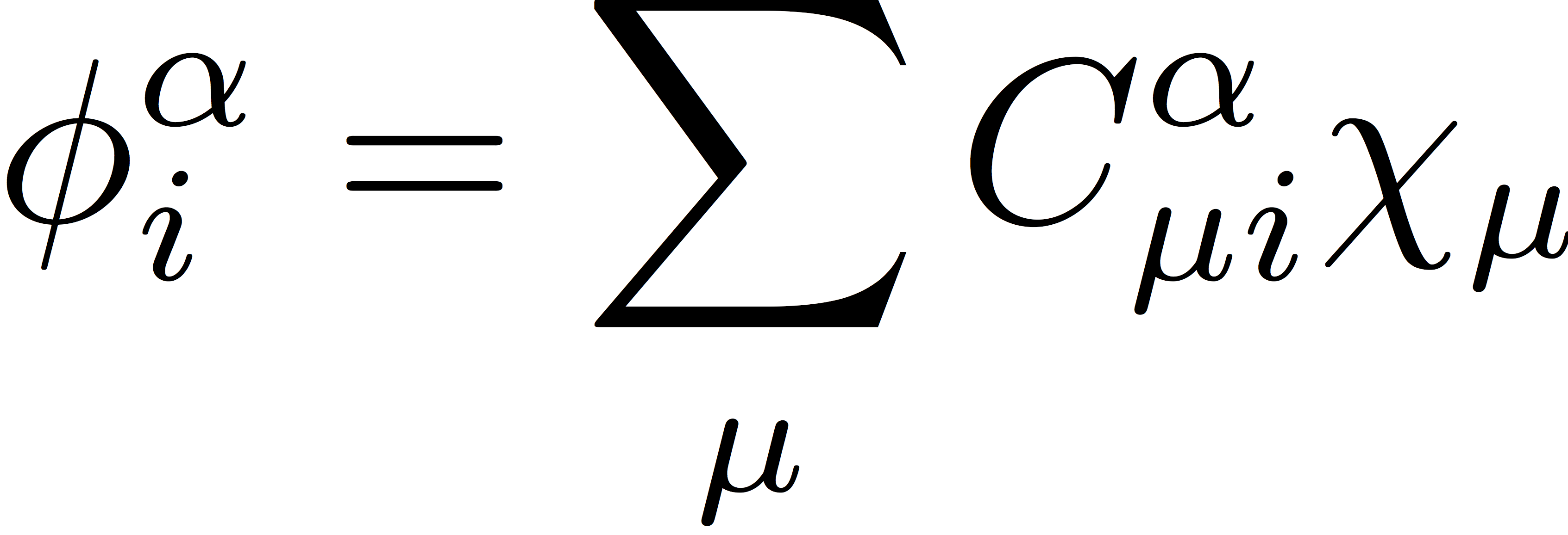
and
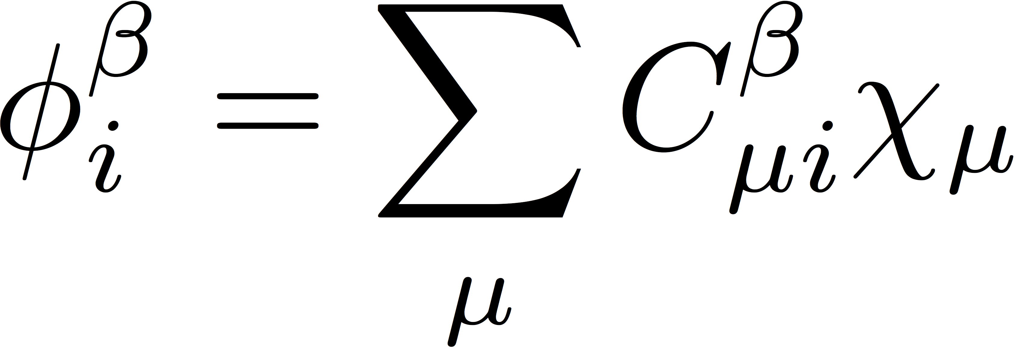
where χμ is an atomic orbital basis function, and the orbital expansion coefficients, Cα and Cβ, are the variable parameters in the SCF procedure. These orbitals then define the α- and β-spin density matrices that are used to construct the Coulomb and exchange matrices. The UHF density matrices are defined as
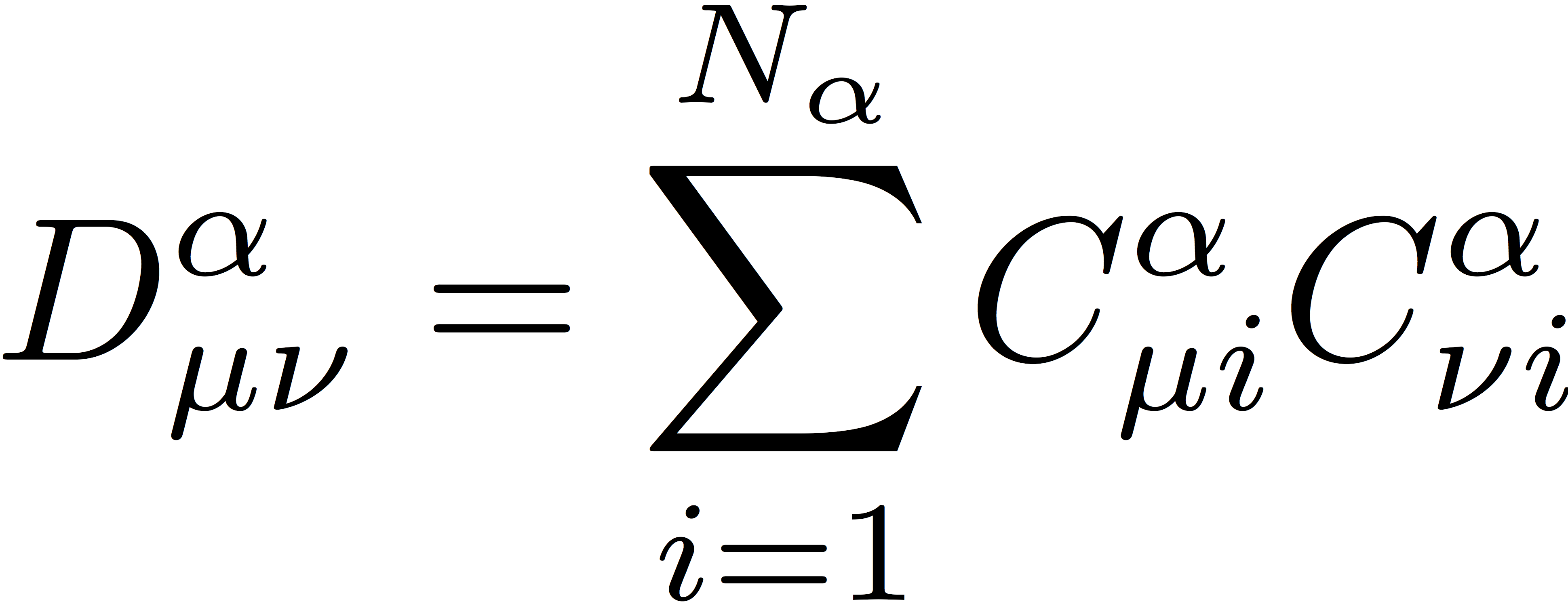
and
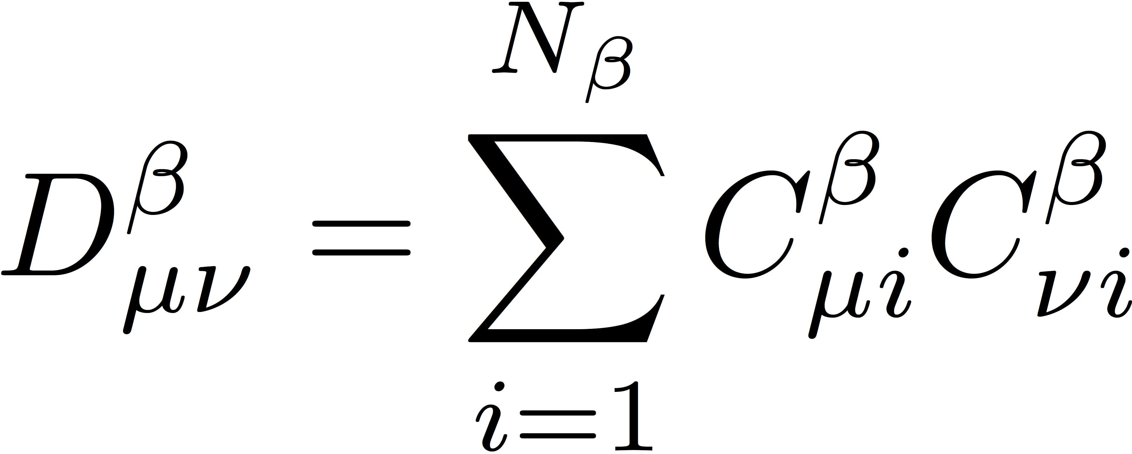
Here, Nα and Nβ represent the number of electrons of α and β spin, respectively. In the previous RHF tutorials, the number of doubly occupied orbitals were determined from the molecule object. Here, we will determine Nα and Nβ in a similar way:
    // use the molecule to determine the total number of electrons
    int charge     = mol->molecular_charge();
    int nelectron  = 0;
    for (int i = 0; i < mol->natom(); i++) {
        nelectron += (int)mol->Z(i);
    }
    nelectron -= charge;

    // use the molecule to determine the multiplicity
    int multiplicity = mol->multiplicity();

    // assuming Ms = S, multiplicity = 2 * Ms + 1
    double ms = (multiplicity - 1 ) / 2;

    // Ms = 1/2 ( Na - Nb )
    // N  = Na + Nb

    int nalpha = ( nelectron + (int)(2 * ms) ) / 2;
    int nbeta  = nelectron - na;
The UHF SCF procedure
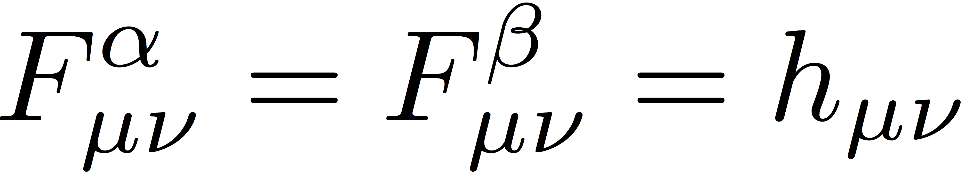
The UHF SCF procedure is similar to the RHF procedure outlined in the previous tutorials. We begin with some guess for the initial orbitals. In the simplest guess, we approximate the α- and β-spin Fock matrices with the core Hamiltonian:
We then transform the Fock matrices to the orthogonal basis defined by Löwdin's symmetric orthogonalization, giving
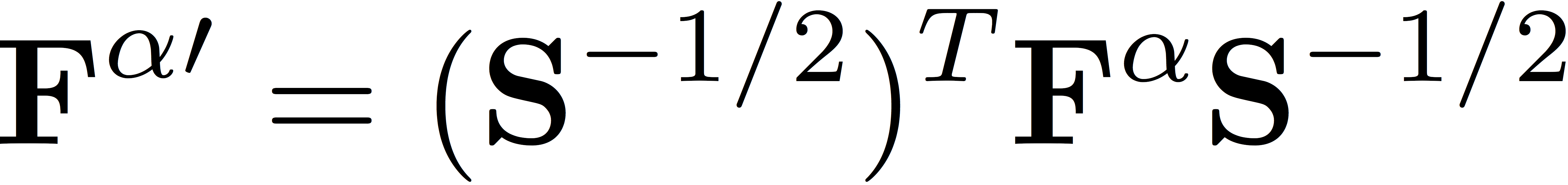
and
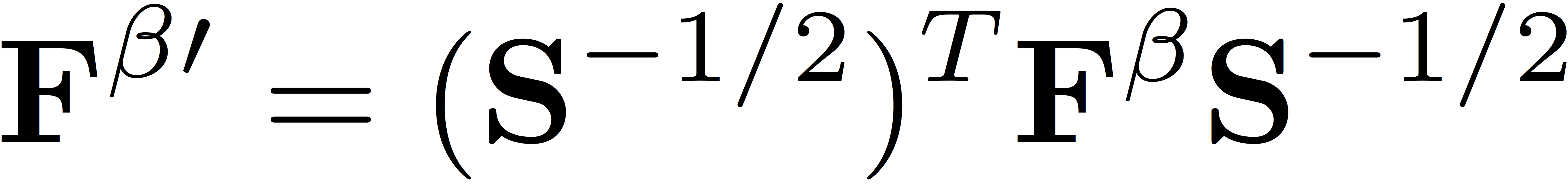
Here, S represents the matrix of overlap integrals. We diagonalize the Fock matrices in the orthogonal basis to determine the eigenvectors

and
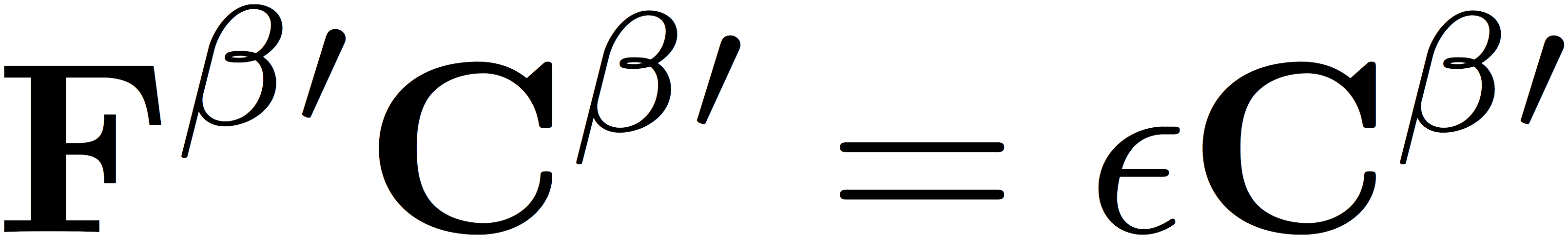
which are related to the orbital coefficients by a partial back transformation to the original non-orthogonal basis, giving
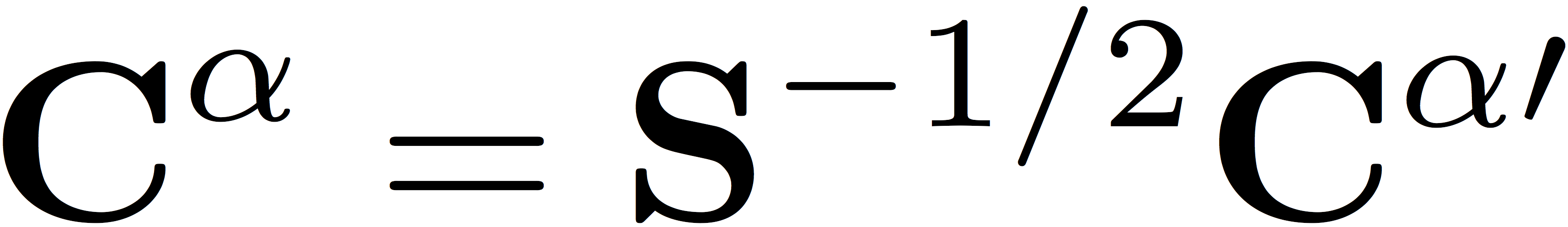
and

When developing your code, you can check your results against some reference data for a modified version of the input file we used in the previous tutorials. Here, we specify that the molecule is a water molecule with a +1 charge.
    molecule {
    1 2
    O
    H 1 R
    H 1 R 2 A

    R = .9
    A = 104.5
    # add this line!
    symmetry c1
    }

    set {
      basis sto-3g
      # add these lines!
      scf_type df
      reference uhf
    }

    energy('myscf')
Note that the reference has been specified as UHF. Check your initial α-spin and β-spin guess orbitals for this case.
Now that we have a guess for the orbitals, we can build the α- and β-spin Fock matrices, which can be transformed to the orthogonal basis and diagonalized to determine new orbitals. The construction of the Coulomb and exchange matrices is simplified when using Psi4's JK object. For UHF, the JK object is initialized in the same way as it was in the case of RHF.
    // JK object
    std::shared_ptr<DiskDFJK> jk = (std::shared_ptr<DiskDFJK>)(new DiskDFJK(primary,auxiliary));

    // memory for jk (say, 80% of what is available)
    jk->set_memory(0.8 * Process::environment.get_memory());

    // integral cutoff
    jk->set_cutoff(options.get_double("INTS_TOLERANCE"));

    // Do J/K, Not wK
    jk->set_do_J(true);
    jk->set_do_K(true);
    jk->set_do_wK(false);

    jk->initialize();
Since we do not (yet) require the wK matrices for range-separated DFT, we initialize the JK object to compute only Coulomb and exchange matrices. During the SCF iterations, the JK object can build both α- and β-spin matrices; the way we achieve this is by passing both α- and β-spin orbital coefficients to the object:
        // grab occupied alpha orbitals (the first nalpha)
        std::shared_ptr<Matrix> myCa (new Matrix(Ca) );
        myCa->zero();

        // grab occupied beta orbitals (the first nbeta)
        std::shared_ptr<Matrix> myCb (new Matrix(Cb) );
        myCb->zero();

        for (int mu = 0; mu < nso; mu++) {
            for (int i = 0; i < nalpha; i++) {
                myCa->pointer()[mu][i] = Ca->pointer()[mu][i];
            }
            for (int i = 0; i < nbeta; i++) {
                myCb->pointer()[mu][i] = Cb->pointer()[mu][i];
            }
        }

        // push occupied orbitals onto JK object
        std::vector< std::shared_ptr<Matrix> >& C_left  = jk->C_left();
        C_left.clear();
        C_left.push_back(myCa);
        C_left.push_back(myCb);

        // form J/K
        jk->compute();

        // form Fa = h + Ja + Jb - Ka
        Fa->copy(h);
        Fa->add(jk->J()[0]);
        Fa->add(jk->J()[1]);
        Fa->subtract(jk->K()[0]);

        // form Fb = h + Ja + Jb - Kb
        Fb->copy(h);
        Fb->add(jk->J()[0]);
        Fb->add(jk->J()[1]);
        Fb->subtract(jk->K()[1]);
The jk->J() and jk->K() functions return standard vectors of matrices; if two sets of orbitals are pushed onto the JK object as was done above, then the first matrix in each standard vector correspondes to α spin, and the second matrix in each vector corresponds to β spin. You can check your α-spin and β-spin Coulomb matrices for the first SCF iteration using the input file given above.
Convergence is monitored in UHF in the same way that it is monitored in RHF. The UHF SCF procedure is considered converged when the energy and orbitals cease to change between iterations or when the orbital gradient becomes sufficiently small. Further, as was done in the previous tutorial, the convergence can be accelerated using the direct inversion of the iterative subspace (DIIS) procedure. If you want to use DIIS here, do not extrapolate the α and β Fock matrices separately. Instead, use a single DIIS extrapolation with vectors of twice the dimension of those used in the RHF-based DIIS tutorial. For the input file given above, the UHF procedure with DIIS should converge the energy and RMS orbital gradient to 12 decimal places in 14 iterations.
    Guess energy:     -110.799510649867

    ==>  Begin SCF Iterations <==

     Iter               energy                   dE          RMS |[F,P]|
        0     -73.388214249092      37.411296400775       0.149136560077
        1     -74.619566509198      -1.231352260106       0.012961155955
        2     -74.624038516225      -0.004472007027       0.001632520945
        3     -74.624158762636      -0.000120246411       0.000744873168
        4     -74.624194647106      -0.000035884471       0.000218448493
        5     -74.624198166251      -0.000003519145       0.000047323689
        6     -74.624198335373      -0.000000169121       0.000007498921
        7     -74.624198339078      -0.000000003706       0.000000402856
        8     -74.624198339087      -0.000000000009       0.000000042562
        9     -74.624198339087      -0.000000000000       0.000000015816
       10     -74.624198339087       0.000000000000       0.000000010050
       11     -74.624198339087       0.000000000000       0.000000000650
       12     -74.624198339087      -0.000000000000       0.000000000006
       13     -74.624198339087       0.000000000000       0.000000000000

    SCF iterations converged!

    * SCF total energy:     -74.624198339087
Unrestricted Kohn-Sham DFT
In Kohn-Sham DFT, we hold that the electronic energy is a universal functional of the one-electron density and, further, there exists a fictitious noninteracting system of electrons that has the same density as the true set of electrons. The states of the fictitious system are determined in a manner that is similar to Hartree-Fock theory; the Kohn-Sham wave function is a single antisymmetrized product of Kohn-Sham orbitals, and these orbitals are determined as the eigenvectors of an effective one-electron operator that accounts for true many-body effects. The unrestricted Kohn-Sham (UKS) energy is

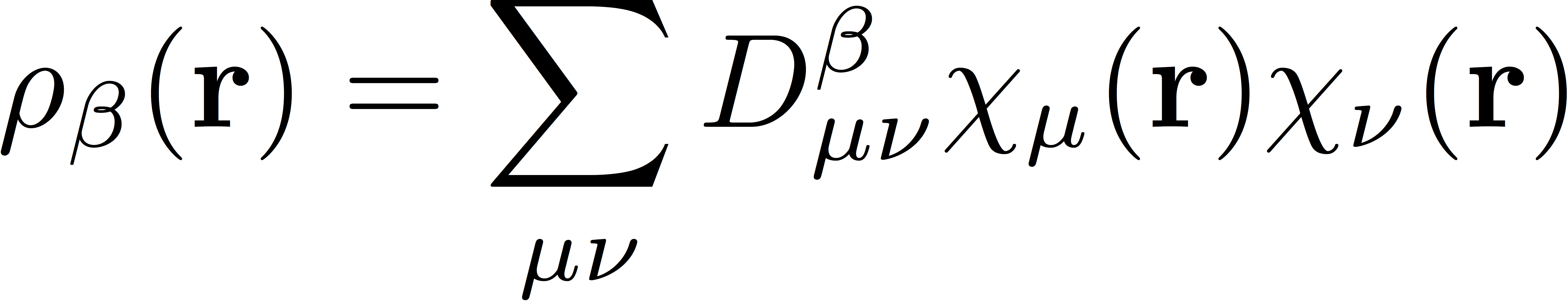
where Exc represents the exchange-correlation energy functional, and ρα and ρβ represent the α and β spin densities, respectively. These spin densities are the real-space representation of the densities, defined as
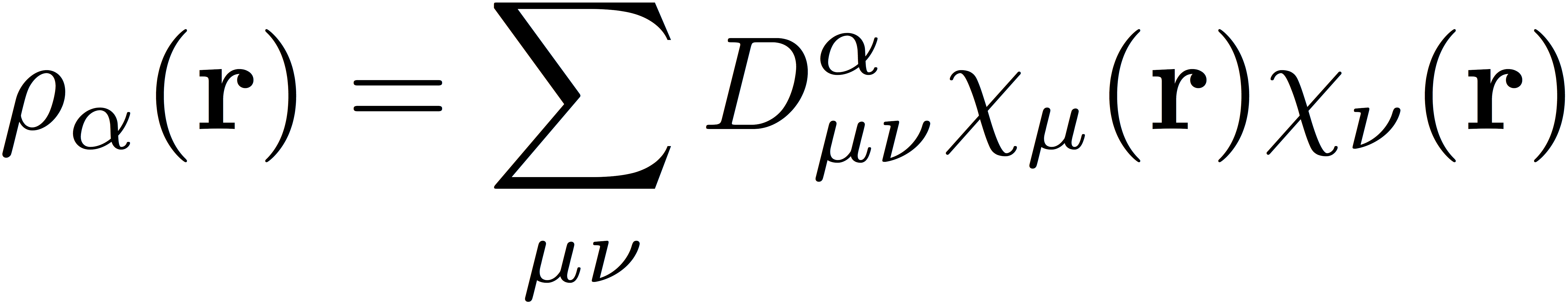
and
The simplest exchange-correlation functionals depend only on the spin densities; these functionals are categorized as Local Spin-Density Approximations (LSDA). Generalized Gradient Approximation (GGA) functionals also depend on the gradient of the spin densities. More complicated functionals can be developed by considering also the second derivative of the spin density (these are meta GGA functionals). Kohn-Sham functionals can be further generalized to include some percentage (usually denoted by α) of "exact" Hartree-Fock exchange; in such "hybrid" functionals, the electronic energy also includes contributions from the usual Hartree-Fock exchange matrices. Lastly, one can also devise so-called long-range corrected (LRC) functionals that use Hartree-Fock exchange at long range and the density functional approximation to exchange at short range; of course, in this case, one much choose some scheme to partition space to distinguish between "short-" and "long-range" interactions. The usual choice is the error function, erf(ωr12), where ω is the range-separation parameter. The general form of the exchange-correlation energy then involves integrals over the exchange-correlation functional and the short/long-range components of the exchange; see the section of the Psi4 manual on DFT for more detail.
In practice, the unrestricted Kohn-Sham DFT orbitals are optimized in a way that is very similar to the UHF procedure. Rather than diagonalizing the UHF Fock matrices to determine our orbitals, we diagonalize Kohn-Sham matrices, which have a similar form

Here, σ represents the spin for the electron (α or β), α represents the percentage of exact Hartree-Fock exchange, Kσ,ω represents an exchange matrix generated with the operator erf(ωr12)/r12, as opposed to the usual Coulomb operator, 1/r12, and Vxc,α represents the exchange-correlation potential matrix, which is comprised of integrals over derivatives of the exchange-correlation functional. For more detail as to what actually goes into Vxc,α, see here.
So! All we need to do to turn our UHF code into a UKS code is figure out how to grab from Psi4 each of the DFT-specific quantities that comprise the Kohn-Sham matrices and energy.
Modifying your UHF code
The first thing we need to do is modify the Python sequence that calls the UHF/UKS plugin in order to be sure that the plugin knows which DFT functional to use. Open the file pymodule.py. Comment out the portions that compute the SCF reference wave function that is passed to the plugin. This reference will not contain any information about the DFT functional for the UKS procedure, so we must create a reference wave function that contains this information. Modify your Python run sequence to match the one given below.
    # Your plugin's psi4 run sequence goes here

    # determine dft functional from options
    func = psi4.core.get_option('MYSCF','FUNCTIONAL')

    # comment out or remove the lines below that compute the
    # scf reference.  we will construct our own wave function.

    # Compute a SCF reference, a wavefunction is return which holds the molecule used, orbitals
    # Fock matrices, and more
    #print('Attention! This SCF may be density-fitted.')

    #ref_wfn = kwargs.get('ref_wfn', None)
    #if ref_wfn is None:
    #    ref_wfn = psi4.driver.scf_helper(name, **kwargs)

    # add these lines below to create a wave function to pass to the plugin

    scf_molecule = kwargs.get('molecule', psi4.core.get_active_molecule())
    base_wfn = psi4.core.Wavefunction.build(scf_molecule, psi4.core.get_global_option('BASIS'))
    scf_wfn = proc.scf_wavefunction_factory(psi4.core.get_option('SCF', 'REFERENCE'), base_wfn, func)


    # Ensure IWL files have been written when not using DF/CD
    proc_util.check_iwl_file_from_scf_type(psi4.core.get_option('SCF', 'SCF_TYPE'), scf_wfn)

    # Call the Psi4 plugin
    # Please note that setting the reference wavefunction in this way is ONLY for plugins
    myscf_wfn = psi4.core.plugin('myscf.so', scf_wfn)
Note that the proc.scf_wavefunction_factory.build() call is not accessible using the standard plugin template generated via "psi4 --plugin-name mydft". At the top of pymodule.py, you must import an additional library as
from psi4.driver.procrouting import proc
Note also that there is a line above asking the options object for information about the functional. This option will be specific to your plugin and needs to be added to the C++ code in the function int read_options(std::string name, Options& options):
        /*- DFT functional -*/
        options.add_str("FUNCTIONAL", "B3LYP");
The default functional will be B3LYP. You will also need to include two additional headers in order to use the DFT functional and potential objects. Add the following headers to your C++ code containing your UHF procedure:
// for dft
#include "psi4/libfock/v.h"
#include "psi4/libfunctional/superfunctional.h"
Find the portion of your code where you initialized your JK object, and add the following lines to determine the functional and to initialize the DFT potential object, before you initialize the JK object:
    // determine the DFT functional and initialize the potential object
    scf::HF* scfwfn = (scf::HF*)ref_wfn.get();
    std::shared_ptr<SuperFunctional> functional = scfwfn->functional();
    std::shared_ptr<VBase> potential =
        VBase::build_V(primary,functional,options,
        (options.get_str("REFERENCE") == "RKS" ? "RV" : "UV"));

    potential->initialize();

    // print the ks information
    potential->print_header();
Now, when initializing the JK object, the functional object can tell us whether or not the JK object needs to compute the exchange matrices necessary for hybrid or LRC functionals:
    // JK object
    std::shared_ptr<DiskDFJK> jk = (std::shared_ptr<DiskDFJK>)(new DiskDFJK(primary,auxiliary));

    // memory for jk (say, 80% of what is available)
    jk->set_memory(0.8 * Process::environment.get_memory());

    // integral cutoff
    jk->set_cutoff(options.get_double("INTS_TOLERANCE"));

    // Do J.
    jk->set_do_J(true);

    // Do K?
    jk->set_do_K(functional->is_x_hybrid());

    // Do wK?
    jk->set_do_wK(functional->is_x_lrc());
    jk->set_omega(functional->x_omega());

    jk->initialize();
With the JK and potential objects properly initialized, we are ready to modify the UHF procedure. Locate the portion of your UHF procedure where the J and K matrices are formed
        // form J/K
        jk->compute();
For every DFT functional, the Fock matrices will include the core Hamiltonian and Coulomb matrices. Ask your functional object if you need to include exact exchange, and do so, if necessary
        // exact exchange?
        if (functional->is_x_hybrid()) {
            // form F -= alpha K
            double alpha = functional->x_alpha();
            Fa->axpy(-alpha,jk->K()[0]);
            Fb->axpy(-alpha,jk->K()[1]);
        }
If you are using a LRC functional, you must also include the exchange matrix generated with the modified erf integrals:
        // LRC functional?
        if (functional->is_x_lrc()) {
            // form Fa/b -= beta wKa/b
            double beta = 1.0 - functional->x_alpha();
            Fa->axpy(-beta,jk->wK()[0]);
            Fb->axpy(-beta,jk->wK()[1]);
        }
Lastly, we will need to include the exchange-correlation potential, which is computed by the potential object. The potential object needs to know the current α and β densities; once you have built these from your occupied α and β orbitals, you can pass them to the potential object using its "set_D" function.
        if (functional->needs_xc()) {

            // set a/b densities in potential object
            potential->set_D({Da_, Db_});

            // evaluate a/b potentials
            potential->compute_V({Va_,Vb_});

            // form Fa/b = h + Ja + Jb + Va/b
            Fa_->add(Va_);
            Fb_->add(Vb_);

        }
Note that Va_ and Vb_ are not members of the Wavefunction class, so you will need to declare and allocate memory for them somewhere. Check your α- and β-spin exchange correlation potential matrices from the first UKS iteration (these matrices correspond to the same molecule and basis set given above and the B3LYP functional).
The remaining steps of the UKS procedure are identical to those of the UHF procedure, with one minor exception. When computing the energy, be sure to check whether or not your functional requires exact exchange or is a range-separated functional, and include those contributions as necessary. The exchange-correlation energy can be grabbed from the potential object as
        double exchange_correlation_energy = 0.0;
        if (functional->needs_xc()) {
            exchange_correlation_energy = potential->quadrature_values()["FUNCTIONAL"];
        }
If everything is working correctly, and you are using DIIS extrapolation, then the UKS procedure should converge to 12 decimal places in 14 iterations:
    Guess energy:     -110.799510649867

    ==>  Begin SCF Iterations <==

     Iter               energy                   dE          RMS |[F,P]|
        0     -73.676857884422      37.122652765444       0.147303908685
        1     -74.626297789124      -0.949439904702       0.096024656906
        2     -74.850040394365      -0.223742605242       0.045441021403
        3     -74.900520282450      -0.050479888085       0.022996151165
        4     -74.916288934361      -0.015768651911       0.000125554060
        5     -74.916289544491      -0.000000610129       0.000014399112
        6     -74.916289560314      -0.000000015823       0.000002548860
        7     -74.916289560844      -0.000000000530       0.000000148231
        8     -74.916289560844      -0.000000000001       0.000000017916
        9     -74.916289560844       0.000000000000       0.000000005593
       10     -74.916289560844       0.000000000000       0.000000004605
       11     -74.916289560844       0.000000000000       0.000000000068
       12     -74.916289560844       0.000000000000       0.000000000006
       13     -74.916289560844      -0.000000000000       0.000000000000

    SCF iterations converged!

    * SCF total energy:     -74.916289560844
This energy should match that from Psi4's DFT using the "energy('b3lyp')" call in your input file.